Making Our Own Types
In the previous chapters, we covered some existing Elm types. In this chapter, we’ll learn how to make our own and how to put them to work!
Algebraic data types intro
So far, we’ve run into a lot of data types. Bool, Int, Char, Maybe, etc.
But how do we make our own? Well, one way is to use the type keyword
to define a type. In the standard library, Bool is translated directly
to JavaScript, but let’s see how we could define our own Bool type.
type Bool = False | True
type means that we’re defining a new data type. The part before the =
denotes the type, which is Bool. The parts after the = are value
constructors. They specify the different values that this type can
have. The | is read as or. So we can read this as: the Bool type can
have a value of True or False. Both the type name and the value
constructors have to be capital cased.
In a similar fashion, we can think of the Int type as being defined like
this:
type Int = -9007199254740991 | -9007199254740990 | ... | -1 | 0 | 1 | 2 | ... | 9007199254740991

The first and last value constructors are the minimum and maximum
possible values of Int. It’s not actually defined like this, the
ellipses are here because we omitted a heapload of numbers, so this is
just for illustrative purposes.
Now, let’s think about how we would represent a shape in Elm. One
way would be to use tuples. A circle could be denoted as (43.1, 55.0,
10.4) where the first and second fields are the coordinates of the
circle’s center and the third field is the radius. Sounds OK, but those
could also represent a 3D vector or anything else. A better solution
would be to make our own type to represent a shape. Let’s say that a
shape can be a circle or a rectangle. Here it is:
type Shape = Circle Float Float Float | Rectangle Float Float Float Float
Now what’s this? Think of it like this. The Circle value constructor has
three fields, which take floats. So when we write a value constructor,
we can optionally add some types after it and those types define the
values it will contain. Here, the first two fields are the coordinates
of its center, the third one its radius. The Rectangle value constructor
has four fields which accept floats. The first two are the coordinates
to its upper left corner and the second two are coordinates to its lower
right one.
Now when I say fields, I actually mean parameters. Value constructors are actually functions that ultimately return a value of a data type. Let’s take a look at the type signatures for these two value constructors.
> Circle
<function> : Float -> Float -> Float -> Shape
> Rectangle
<function> : Float -> Float -> Float -> Float -> Shape
Cool, so value constructors are functions like everything else. Who would have thought? Let’s make a function that takes a shape and returns its surface.
surface : Shape -> Float
surface s = case s of
  (Circle _ _ r) -> pi * r ^ 2
  (Rectangle x1 y1 x2 y2) -> (abs <| x2 - x1) * (abs <| y2 - y1)
The first notable thing here is the type declaration. It says that the
function takes a shape and returns a float. We couldn’t write a type
declaration of Circle -> Float because Circle is not a type, Shape is.
Just like we can’t write a function with a type declaration of True ->
Int. The next thing we notice here is that we can pattern match against
constructors. We pattern matched against constructors before (all the
time actually) when we pattern matched against values like "string" or False
or 5, only those values didn’t have any fields. We just write a
constructor and then bind its fields to names. Because we’re interested
in the radius, we don’t actually care about the first two fields, which
tell us where the circle is.
> surface <| Circle 10 20 10
314.1592653589793 : Float
> surface <| Rectangle 0 0 100 100
10000 : Float
Yay, it works! Value constructors are functions, so we can map them and partially apply them and everything. If we want a list of concentric circles with different radii, we can do this.
> List.map (Circle 10 20) [4,5,6,7]
[Circle 10.0 20.0 4.0,Circle 10.0 20.0 5.0,Circle 10.0 20.0 6.0,Circle 10.0 20.0 7.0] : List Shape
Our data type is good, although it could be better. Let’s make an intermediate data type that defines a point in two-dimensional space. Then we can use that to make our shapes more understandable.
type Point = Point Float Float
type Shape = Circle Point Float | Rectangle Point Point
Notice that when defining a point, we used the same name for the data
type and the value constructor. This has no special meaning, although
it’s common to use the same name as the type if there’s only one value
constructor. So now the Circle has two fields, one is of type Point and
the other of type Float. This makes it easier to understand what’s what.
Same goes for the rectangle. We have to adjust our surface function to
reflect these changes.
surface : Shape -> Float
surface s = case s of
  (Circle _ r) -> pi * r ^ 2
  (Rectangle (Point x1 y1) (Point x2 y2)) -> (abs <| x2 - x1) * (abs <| y2 - y1)
The only thing we had to change were the patterns. We disregarded the whole point in the circle pattern. In the rectangle pattern, we just used a nested pattern matching to get the fields of the points. If we wanted to reference the points themselves for some reason, we could have used as-patterns.
> surface (Rectangle (Point 0 0) (Point 100 100))
10000 : Float
> surface (Circle (Point 0 0) 24)
1809.5574 : Float
How about a function that nudges a shape? It takes a shape, the amount to move it on the x axis and the amount to move it on the y axis and then returns a new shape that has the same dimensions, only it’s located somewhere else.
nudge : Shape -> Float -> Float -> Shape
nudge s a b = case s of
  (Circle (Point x y) r) -> Circle (Point (x+a) (y+b)) r
  (Rectangle (Point x1 y1) (Point x2 y2)) -> Rectangle (Point (x1+a) (y1+b)) (Point (x2+a) (y2+b))
Pretty straightforward. We add the nudge amounts to the points that denote the position of the shape.
> nudge (Circle (Point 34 34) 10) 5 10
Circle (Point 39.0 44.0) 10.0 : Shape
If we don’t want to deal directly with points, we can make some auxilliary functions that create shapes of some size at the zero coordinates and then nudge those.
baseCircle : Float -> Shape
baseCircle r = Circle (Point 0 0) r

baseRect : Float -> Float -> Shape
baseRect width height = Rectangle (Point 0 0) (Point width height)
> nudge (baseRect 40 100) 60 23
Rectangle (Point 60.0 23.0) (Point 100.0 123.0) : Shape
You can, of course, export your data types in your modules. To do that,
just write your type along with the functions you are exporting and then
add some parentheses and in them specify the value constructors that you
want to export for it, separated by commas. If you want to export all
the value constructors for a given type, just write ..
If we wanted to export the functions and types that we defined here in a module, we could start it off like this:
module Shapes exposing
    ( Point(..)
    , Shape(..)
    , surface
    , nudge
    , baseCircle
    , baseRect
    )
By doing Shape(..), we exported all the value constructors for Shape, so
that means that whoever imports our module can make shapes by using the
Rectangle and Circle value constructors. It’s the same as writing Shape
(Rectangle, Circle).
We could also opt not to export any value constructors for Shape by just
writing Shape in the export statement. That way, someone importing our
module could only make shapes by using the auxilliary functions
baseCircle and baseRect. Set uses that approach. You can’t create a
set by doing Set.Set [(1,2),(3,4)] because it doesn’t export that value
constructor. However, you can make a set by using one of the
auxilliary functions like Set.fromList. Remember, value constructors are
just functions that take the fields as parameters and return a value of
some type (like Shape) as a result. So when we choose not to export
them, we just prevent the person importing our module from using those
functions, but if some other functions that are exported return a type,
we can use them to make values of our custom data types.
Not exporting the value constructors of a data types makes them more abstract in such a way that we hide their implementation. Also, whoever uses our module can’t pattern match against the value constructors.
Record syntax
OK, we’ve been tasked with creating a data type that describes a person. The info that we want to store about that person is: first name, last name, age, height, phone number, and favorite ice-cream flavor. I don’t know about you, but that’s all I ever want to know about a person. Let’s give it a go!
type Person = Person String String Int Float String String
O-kay. The first field is the first name, the second is the last name, the third is the age and so on. Let’s make a person.
> guy = Person "Buddy" "Finklestein" 43 184.2 "526-2928" "Chocolate"
Person "Buddy" "Finklestein" 43 184.2 "526-2928" "Chocolate" : Person
That’s kind of cool, although slightly unreadable. What if we want to create a function to get seperate info from a person? A function that gets some person’s first name, a function that gets some person’s last name, etc. Well, we’d have to define them kind of like this.
firstName : Person -> String
firstName (Person firstname _ _ _ _ _) = firstname

lastName : Person -> String
lastName (Person _ lastname _ _ _ _) = lastname

age : Person -> Int
age (Person _ _ age _ _ _) = age

height : Person -> Float
height (Person _ _ _ height _ _) = height

phoneNumber : Person -> String
phoneNumber (Person _ _ _ _ number _) = number

flavor : Person -> String
flavor (Person _ _ _ _ _ flavor) = flavor
Whew! I certainly did not enjoy writing that! Despite being very cumbersome and BORING to write, this method works.
> guy = Person "Buddy" "Finklestein" 43 184.2 "526-2928" "Chocolate"
Person "Buddy" "Finklestein" 43 184.2 "526-2928" "Chocolate" : Person
> firstName guy
"Buddy" : String
> height guy
184.2 : Float
> flavor guy
"Chocolate" : String
There must be a better way, you say! Well no, there isn’t, sorry.
Just kidding, there is. Hahaha! The makers of Elm were very smart and anticipated this scenario. They included an alternative way to write data types. Here’s how we could achieve the above functionality with record syntax.
type Person = Person { firstName : String
                     , lastName : String
                     , age : Int
                     , height : Float
                     , phoneNumber : String
                     , flavor : String
                     }
So instead of just naming the field types one after another and
separating them with spaces, we use curly brackets. First we write the
name of the field, for instance, firstName and then we write a
colon : and then we specify
the type. The resulting data type is exactly the same. The main benefit
of this is that it creates functions that lookup fields in the data
type. By using record syntax to create this data type, Elm
automatically made these functions: .firstName, .lastName, .age,
.height, .phoneNumber and .flavor.
> flavor
<function> : { b | flavor : a } -> a
> firstName
<function> : { b | firstName : a } -> a
There’s another benefit to using record syntax. When we print the the type, it displays it differently if we use record syntax to define and instantiate the type. Say we have a type that represents a car. We want to keep track of the company that made it, the model name and its year of production. Watch.
type Car = Car String String Int
> Car "Ford" "Mustang" 1967
Car "Ford" "Mustang" 1967 : Car
If we define it using record syntax, we can make a new car like this.
type Car = Car {company : String, model : String, year : Int}
> Car {company="Ford", model="Mustang", year=1967}
Car { company = "Ford", model = "Mustang", year = 1967 } : Car
When making a new car, we don’t have to necessarily put the fields in the proper order, as long as we list all of them. But if we don’t use record syntax, we have to specify them in order.
Use record syntax when a constructor has several fields and it’s not
obvious which field is which. If we make a 3D vector data type by doing
type Vector = Vector Int Int Int, it’s pretty obvious that the fields
are the components of a vector. However, in our Person and Car types, it
wasn’t so obvious and we greatly benefited from using record syntax.
Type parameters
A value constructor can take some values parameters and then produce a
new value. For instance, the Car constructor takes three values and
produces a car value. In a similar manner, type constructors can take
types as parameters to produce new types. This might sound a bit too
meta at first, but it’s not that complicated. If you’re familiar with
templates in C++, you’ll see some parallels. To get a clear picture of
what type parameters work like in action, let’s take a look at how a
type we’ve already met is implemented.
type Maybe a = Nothing | Just a
The a here is the type parameter. And because there’s a type parameter
involved, we call Maybe a type constructor. Depending on what we want
this data type to hold when it’s not Nothing, this type constructor can
end up producing a type of Maybe Int, Maybe Car, Maybe String, etc. No
value can have a type of just Maybe, because that’s not a type per se,
it’s a type constructor. In order for this to be a real type that a
value can be part of, it has to have all its type parameters filled up.
So if we pass Char as the type parameter to Maybe, we get a type of
Maybe Char. The value Just 'a' has a type of Maybe Char, for example.
You might not know it, but we used a type that has a type parameter
before we used Maybe. That type is the list type. The list type takes
a parameter to produce a concrete type. Values can have a List Int type,
a List Char type, a List (List String) type, but you can’t have a value
that just has a type of List.
Let’s play around with the Maybe type.
> Just "Haha"
Just "Haha" : Maybe String
> Just 84
Just 84 : Maybe number
> Nothing
Nothing : Maybe a
> Just 10.0
Just 10.0 : Maybe Float
Type parameters are useful because we can make different types with them
depending on what kind of types we want contained in our data type. When
we do Just "Haha", the type inference engine figures it out to be of
the type Maybe String, because if the a in the Just a is a string, then
the a in Maybe a must also be a string.
Notice that the type of Nothing is Maybe a. Its type is polymorphic. If
some function requires a Maybe Int as a parameter, we can give it a
Nothing, because a Nothing doesn’t contain a value anyway and so it
doesn’t matter. The Maybe a type can act like a Maybe Int if it has to,
just like 5 can act like an Int or a Double. Similarly, the type of the
empty list is List a. An empty list can act like a list of anything. That’s
why we can do [1,2,3] ++ [] and ["ha","ha","ha"] ++ [].
Using type parameters is very beneficial, but only when using them makes
sense. Usually we use them when our data type would work regardless of
the type of the value it then holds inside it, like with our Maybe a
type. If our type acts as some kind of box, it’s good to use them. We
could change our Car data type from this:
type Car = Car { company : String
               , model : String
               , year : Int
               }
To this:
type Car a b c = Car { company : a
                     , model : b
                     , year : c
                     }
But would we really benefit? The answer is: probably no, because we’d
just end up defining functions that only work on the Car String String
Int type. For instance, given our first definition of Car, we could make
a function that displays the car’s properties in a nice little text.
tellCar : Car -> String
tellCar (Car {company, model, year}) =
  "This " ++ company ++ " " ++
  model ++ " was made in " ++ toString year
> stang = Car {company="Ford", model="Mustang", year=1967}
Car { company = "Ford", model = "Mustang", year = 1967 } : Car
> tellCar stang
"This Ford Mustang was made in 1967" : String
A cute little function! The type declaration is cute and it works
nicely. Now what if Car was Car a b c?
tellCar : Car String String a -> String
tellCar (Car {company, model, year}) =
  "This " ++ company ++ " " ++ model ++ " was made in " ++ toString year
We’d have to force this function to take a Car type of Car
String String a. You can see that the type signature is more complicated
and the only benefit we’d actually get would be that we can use any type
as the type for c.
> tellCar (Car "Ford" "Mustang" 1967)
"This Ford Mustang was made in 1967" : String
> tellCar (Car "Ford" "Mustang" )
"This Ford Mustang was made in \"nineteen sixty seven\"" : String

In real life though, we’d end up using Car String String Int most of the
time and so it would seem that parameterizing the Car type isn’t really
worth it. We usually use type parameters when the type that’s contained
inside the data type’s various value constructors isn’t really that
important for the type to work. A list of stuff is a list of stuff and
it doesn’t matter what the type of that stuff is, it can still work. If
we want to sum a list of numbers, we can specify later in the summing
function that we specifically want a list of numbers. Same goes for
Maybe. Maybe represents an option of either having nothing or having one
of something. It doesn’t matter what the type of that something is.
Another example of a parameterized type that we’ve already met is Dict k
v. The k is the type of the keys in a dictionary and the v is the
type of the values. This is a good example of where type parameters are
very useful. Having dictionaries parameterized enables us to have mappings from
any type to any other type, as long as the type of the key is some comparable
type. If we were defining a mapping type, we could add such a
constraint in the type declaration:
type Dict comparable v = ...
However, it’s a very strong convention in Elm to never add
such constraints in data declarations. Why? Well, because we don’t
benefit a lot, but we end up writing more class constraints, even when
we don’t need them. If we put or don’t put the comparable constraint in the
*type declaration for Dict k v, we’re going to have to put the
constraint into functions that assume the keys in a dictionary can be ordered.
But if we don’t put the constraint in the data declaration, we don’t
have to put comparable in the type declarations of functions that don’t
care whether the keys can be ordered or not. An example of such a
function is toList, that just takes a mapping and converts it to an
associative list. Its type signature is toList : Dict k a -> [(k, a)].
If Dict k v had a type constraint in its type declaration, the type for
toList would have to be toList : Dict comparable v -> List (comparable, v)`, even
though the function doesn’t do any comparing of keys by order.
So don’t put type constraints into type declarations even if it seems to make sense, because you’ll have to put them into the function type declarations either way.
Let’s implement a 3D vector type and add some operations for it. We’ll be using a parameterized type because even though it will usually contain numeric types, it will still support several of them.
type Vector a = Vector a a a

vplus : Vector number -> Vector number -> Vector number
vplus (Vector i j k) (Vector l m n) = Vector (i+l) (j+m) (k+n)

vectMult : Vector number -> number -> Vector number
vectMult (Vector i j k) m = Vector (i*m) (j*m) (k*m)

scalarMult : Vector number -> Vector number -> number
scalarMult (Vector i j k) (Vector l m n) = i*l + j*m + k*n
vplus is for adding two vectors together. Two vectors are added just by
adding their corresponding components. scalarMult is for the scalar
product of two vectors and vectMult is for multiplying a vector with a
scalar. These functions can operate on types of Vector Int, or
Vector Float, as long as the a from Vector a is from the
the number typeclass. Notice that we didn’t put a number class constraint in the
type declaration, because we’d have to repeat it in the functions
anyway.
Once again, it’s very important to distinguish between the type
constructor and the value constructor. When declaring a data type, the
part before the = is the type constructor and the constructors after it
(possibly separated by |’s) are value constructors. Giving a function a
type of Vector t t t -> Vector t t t -> t would be wrong, because we
have to put types in type declaration and the vector type constructor
takes only one parameter, whereas the value constructor takes three.
Let’s play around with our vectors.
> vplus (Vector 3 5 8) (Vector 9 2 8)
Vector 12 7 16 : Vector number
> vplus (Vector 3 5 8) (Vector 9 2 8) |> vplus (Vector 0 2 3)
Vector 12 9 19 : Vector number
> vectMult (Vector 3 9 7) 10
Vector 30 90 70 : Vector number
> scalarMult (Vector 4 9 5) (Vector 9.0 2.0 4.0)
74 : Float
> vectMult (Vector 2 9 3) (scalarMult (Vector 4 9 5) (Vector 9 2 4))
Vector 148 666 222 : Vector number
Type aliases
Type aliases are a way to make your type annotations easier to read.
Type aliases don’t really do anything per se, they’re just
about giving some types different names so that they make more sense to
someone reading our code and documentation. E.g. here’s how the standard
library defines Time as a synonym for Float.
type alias Time = Float
If we make a function that converts a timestamp to an ISO8601 date string
and call it
toISOString or something, we can give it a type declaration of
toISOString : Float -> String or toISOString : Time ->
String. Both of these are essentially the same, only the latter is nicer
to read.
When we were dealing with the Dict module, we first represented a
phonebook with an association list before converting it into a dictionary. As
we’ve already found out, an association list is a list of key-value
pairs. Let’s look at a phonebook that we had.
phoneBook : List (String, String)
phoneBook =
    [("betty","555-2938")
    ,("bonnie","452-2928")
    ,("patsy","493-2928")
    ,("lucille","205-2928")
    ,("wendy","939-8282")
    ,("penny","853-2492")
    ]
We see that the type of phoneBook is List (String,String). That tells us
that it’s an association list that maps from strings to strings, but not
much else. Let’s make a type alias to convey some more information in
the type declaration.
type alias PhoneBook = List (String,String)
Now the type declaration for our phonebook can be phoneBook :
PhoneBook. Let’s make a type alias for String as well.
type alias PhoneNumber = String
type alias Name = String
type alias PhoneBook = List (Name,PhoneNumber)
Giving the String type alias is something that Elm programmers do
when they want to convey more information about what strings in their
functions should be used as and what they represent.
So now, when we implement a function that takes a name and a number and sees if that name and number combination is in our phonebook, we can give it a very pretty and descriptive type declaration.
inPhoneBook : Name -> PhoneNumber -> PhoneBook -> Bool
inPhoneBook name pnumber pbook = List.member (name,pnumber) pbook
If we decided not to use type aliases, our function would have a type
of String -> String -> [(String,String)] -> Bool. In this case, the
type declaration that took advantage of type aliases is easier to
understand. However, you shouldn’t go overboard with them. We introduce
type aliases either to describe what some existing type represents in
our functions (and thus our type declarations become better
documentation) or when something has a long-ish type that’s repeated a
lot (like List (String,String)) but represents something more specific in
the context of our functions.
Type aliases can also be parameterized. If we want a type that represents an association list type but still want it to be general so it can use any type as the keys and values, we can do this:
type alias AssocList comparable v = List (comparable,v)
Now, a function that gets the value by a key in an association list can
have a type of k -> AssocList comparable v -> Maybe v. AssocList is
a type constructor that takes two types and produces a concrete type,
like AssocList Int String, for instance.
Fonzie says: Aaay! When I talk about concrete types I mean like
fully applied types like Map Int String or if we’re dealin’ with one of
them polymorphic functions, List a or Maybe a and stuff. And
like, sometimes me and the boys say that Maybe is a type, but we don’t
mean that, cause every idiot knows Maybe is a type constructor. When I
apply an extra type to Maybe, like Maybe String, then I have a concrete
type. You know, values can only have types that are concrete types! So
in conclusion, live fast, love hard and don’t let anybody else use your
comb!
Make sure that you really understand the distinction between type
constructors and value constructors. Just because we made a type alias
called AssocList doesn’t mean that we can do stuff like
AssocList [(1,2),(4,5),(7,9)]. All it means is that we can refer to its
type by using different names. We can do:
list : AssocList Int Int
list = [(1,2),(3,5),(8,9)]
which will make the numbers inside assume a type of
Int, but we can still use that list as we would any normal list that has
pairs of integers inside. Type aliases (and types generally) can only
be used in the type portion of Elm. We’re in Elm’s type portion
whenever we’re defining new types (so in type and type alias declarations)
or when we’re located after a :. The : is in type declarations or in
type annotations.
Another cool data type that takes two types as its parameters is the
Either a b type. This is roughly how it’s defined:
type Result error value = Ok value | Err error
It has two value constructors. If the Ok is used, then its contents
are of type value and if Err is used, then its contents are of type error.
So we can use this type to encapsulate a value of one type or another and
then when we get a value of type Result error value, we usually pattern match on
both Ok and Err and we do different stuff based on which one of them it
was.
> Ok 20
Ok 20 : Result error number
> Err "w00t"
Err "w00t" : Result String value
So far, we’ve seen that Maybe a was mostly used to represent the results
of computations that could have either failed or not. But somtimes,
Maybe a isn’t good enough because Nothing doesn’t really convey much
information other than that something has failed. That’s cool for
functions that can fail in only one way or if we’re just not interested
in how and why they failed. A Dict lookup fails only if the key we
were looking for wasn’t in the dictionary, so we know exactly what happened.
However, when we’re interested in how some function failed or why, we
usually use the result type of Result error value, where error is some sort of type
that can tell us something about the possible failure and value is the type
of a successful computation. Hence, errors use the Err value
constructor while results use Ok.
An example: a high-school has lockers so that students have some place
to put their Guns’n’Roses posters. Each locker has a code combination.
When a student wants a new locker, they tell the locker supervisor which
locker number they want and he gives them the code. However, if someone
is already using that locker, he can’t tell them the code for the locker
and they have to pick a different one. We’ll use a dictionary from Dict to
represent the lockers. It’ll map from locker numbers to a pair of
whether the locker is in use or not and the locker code.
import Dict

type LockerState = Taken | Free

type alias Code = String

type alias LockerMap = Dict.Dict Int (LockerState, Code)
Simple stuff. We introduce a new data type to represent whether a locker is taken or free and we make a type synonym for the locker code. We also make a type synonym for the type that maps from integers to pairs of locker state and code. And now, we’re going to make a function that searches for the code in a locker dictionary. We’re going to use an Either String Code type to represent our result, because our lookup can fail in two ways — the locker can be taken, in which case we can’t tell the code or the locker number might not exist at all. If the lookup fails, we’re just going to use a String to tell what’s happened.
lockerLookup : Int -> LockerMap -> Result String Code
lockerLookup lockerNumber dict =
    case Dict.get lockerNumber dict of
        Nothing -> Err <| "Locker number " ++ toString lockerNumber ++ " doesn't exist!"
        Just (state, code) -> if state /= Taken
                                then Ok code
                                else Err <| "Locker " ++ toString lockerNumber ++ " is already taken!"
We do a normal lookup in the dictionary. If we get a Nothing, we return a value
of type Err String, saying that the locker doesn’t exist at all. If we
do find it, then we do an additional check to see if the locker is
taken. If it is, return an Err saying that it’s already taken. If it
isn’t, then return a value of type Ok Code, in which we give the
student the correct code for the locker. It’s actually an Ok String,
but we introduced that type alias to introduce some additional
documentation into the type declaration. Here’s an example dictionary:
lockers : LockerMap
lockers = Dict.fromList
    [(100,(Taken,"ZD39I"))
    ,(101,(Free,"JAH3I"))
    ,(103,(Free,"IQSA9"))
    ,(105,(Free,"QOTSA"))
    ,(109,(Taken,"893JJ"))
    ,(110,(Taken,"99292"))
    ]
Now let’s try looking up some locker codes.
> lockerLookup 101 lockers
Ok "JAH3I" : Result String Code
> lockerLookup 100 lockers
Err "Locker 100 is already taken!" : Result String Code
> lockerLookup 102 lockers
Err "Locker number 102 doesn't exist!" : Result String Code
> lockerLookup 110 lockers
Err "Locker 110 is already taken!" : Result String Code
> lockerLookup 105 lockers
Ok "QOTSA" : Result String Code
We could have used a Maybe a to represent the result but then we
wouldn’t know why we couldn’t get the code. But now, we have information
about the failure in our result type.
Recursive data structures

As we’ve seen, a constructor in an algebraic data type can have several (or none at all) fields and each field must be of some concrete type. With that in mind, we can make types whose constructors have fields that are of the same type! Using that, we can create recursive data types, where one value of some type contains values of that type, which in turn contain more values of the same type and so on.
Think about this list: [5]. That’s just syntactic sugar for 5::[]. On the
left side of the ::, there’s a value and on the right side, there’s a
list. And in this case, it’s an empty list. Now how about the list
[4,5]? Well, that desugars to 4::(5::[]). Looking at the first ::, we see
that it also has an element on its left side and a list (5::[]) on its
right side. Same goes for a list like 3::(4::(5::6::[])), which could be
written either like that or like 3::4::5::6::[] (because :: is
right-associative) or [3,4,5,6].
We could say that a list can be an empty list or it can be an element
joined together with a :: with another list (that can be either the empty
list or not).
Let’s use algebraic data types to implement our own list then!
type List a = Empty | Cons a (List a)
This reads just like our definition of lists from one of the previous paragraphs. It’s either an empty list or a combination of a head with some value and a list. If you’re confused about this, you might find it easier to understand in record syntax.
type List a = Empty | Cons { listHead : a, listTail : List a}
You might also be confused about the Cons constructor here. cons is
another word for ::. You see, in lists, :: is actually a constructor that
takes a value and another list and returns a list. We can already use
our new list type! In other words, it has two fields. One field is of
the type of a and the other is of the type List a.
> Empty
Empty : List a
> Cons 5 Empty
Cons 5 Empty : List number
> Cons 4 (Cons 5 Empty)
Cons 4 (Cons 5 Empty) : List number
> Cons 3 (Cons 4 (Cons 5 Empty))
Cons 3 (Cons 4 (Cons 5 Empty)) : List number
Let’s make a function that adds two of our lists together. This is how ++ is defined for normal lists:
(+++) : List a -> List a -> List a
(+++) ls rs = case ls of
    [] -> rs
    (x::xs) -> x :: (xs +++ rs)

infixr 5 +++
First off, we notice a new syntactic construct, the fixity declarations.
We can define functions to be automatically infix by making them
comprised of only special characters. (In the example above, we made our own
operator +++ instead of trying to redefine the existing ++, because
elm only allows fixity to be set once).
When we define functions as operators, we can use that to give them a
fixity (but we don’t have to). A fixity states how tightly the operator
binds and whether it’s left-associative or right-associative. For
instance, *’s fixity is infixl 7 * and +’s fixity is infixl 6. That
means that they’re both left-associative (4 * 3 * 2 == (4 * 3) * 2)
but * binds tighter than +, because it has a greater fixity, so
5 * 4 + 3 == (5 * 4) + 3.
So we’ll just steal that for our own list. We’ll name the function .++.
(.++) : List a -> List a -> List a
(.++) ls rs = case ls of
    Empty -> rs
    Cons x xs -> Cons x (xs .++ rs)

infixr 5 .++
And let’s see if it works …
> a = Cons 3 (Cons 4 (Cons 5 Empty))
Cons 3 (Cons 4 (Cons 5 Empty)) : List number
> b = Cons 6 (Cons 7 Empty)
b = Cons 6 (Cons 7 Empty) : List number
> a .++ b
Cons 3 (Cons 4 (Cons 5 (Cons 6 (Cons 7 Empty)))) : List number
Nice. Is nice. If we wanted, we could implement all of the functions that operate on lists on our own list type.
Now, we’re going to implement a binary search tree. If you’re not familiar with binary search trees from languages like C, here’s what they are: an element points to two elements, one on its left and one on its right. The element to the left is smaller, the element to the right is bigger. Each of those elements can also point to two elements (or one, or none). In effect, each element has up to two sub-trees. And a cool thing about binary search trees is that we know that all the elements at the left sub-tree of, say, 5 are going to be smaller than 5. Elements in its right sub-tree are going to be bigger. So if we need to find if 8 is in our tree, we’d start at 5 and then because 8 is greater than 5, we’d go right. We’re now at 7 and because 8 is greater than 7, we go right again. And we’ve found our element in three hops! Now if this were a normal list (or a tree, but really unbalanced), it would take us seven hops instead of three to see if 8 is in there.
Sets and dictionaries (i.e. Set and Dict) are implemented using trees,
only instead of normal binary search trees, they use balanced binary
search trees, which are always balanced. But right now, we’ll just be
implementing normal binary search trees.
Here’s what we’re going to say: a tree is either an empty tree or it’s an element that contains some value and two trees. Sounds like a perfect fit for an algebraic data type!
type Tree a = EmptyTree | Node a (Tree a) (Tree a)
Okay, good, this is good. Instead of manually building a tree, we’re going to make a function that takes a tree and an element and inserts an element. We do this by comparing the value we want to insert to the root node and then if it’s smaller, we go left, if it’s larger, we go right. We do the same for every subsequent node until we reach an empty tree. Once we’ve reached an empty tree, we just insert a node with that value instead of the empty tree.
In languages like C, we’d do this by modifying the pointers and values
inside the tree. In Elm, we can’t really modify our tree, so we have
to make a new sub-tree each time we decide to go left or right and in
the end the insertion function returns a completely new tree, because
Elm doesn’t really have a concept of pointer, just values. Hence,
the type for our insertion function is going to be something like a ->
Tree a - > Tree a. It takes an element and a tree and returns a new
tree that has that element inside.
So, here are two functions. One is a utility function for making a singleton tree (a tree with just one node) and a function to insert an element into a tree.
singleton : a -> Tree a
singleton x = Node x EmptyTree EmptyTree

treeInsert : comparable -> Tree comparable -> Tree comparable
treeInsert x t = case t of
    EmptyTree -> singleton x
    (Node a left right) ->
         if x == a then Node x left right
         else if x < a then Node a (treeInsert x left) right
         else Node a left (treeInsert x right)
The singleton function is just a shortcut for making a node that has
something and then two empty sub-trees. In the insertion function, we
first have the edge condition as a pattern. If we’ve reached an empty
sub-tree, that means we’re where we want and instead of the empty tree,
we put a singleton tree with our element. If we’re not inserting into an
empty tree, then we have to check some things. First off, if the element
we’re inserting is equal to the root element, just return a tree that’s
the same. If it’s smaller, return a tree that has the same root value,
the same right sub-tree but instead of its left sub-tree, put a tree
that has our value inserted into it. Same (but the other way around)
goes if our value is bigger than the root element.
Next up, we’re going to make a function that checks if some element is in the tree. First, let’s define the edge condition. If we’re looking for an element in an empty tree, then it’s certainly not there. Okay. Notice how this is the same as the edge condition when searching for elements in lists. If we’re looking for an element in an empty list, it’s not there. Anyway, if we’re not looking for an element in an empty tree, then we check some things. If the element in the root node is what we’re looking for, great! If it’s not, what then? Well, we can take advantage of knowing that all the left elements are smaller than the root node. So if the element we’re looking for is smaller than the root node, check to see if it’s in the left sub-tree. If it’s bigger, check to see if it’s in the right sub-tree.
treeElem : comparable -> Tree comparable -> Bool
treeElem x t = case t of
    EmptyTree -> False
    (Node a left right) ->
        if x == a then True
        else if x < a then treeElem x left
        else treeElem x right
All we had to do was write up the previous paragraph in code. Let’s have some fun with our trees! Instead of manually building one (although we could), we’ll use a fold to build up a tree from a list. Remember, pretty much everything that traverses a list one by one and then returns some sort of value can be implemented with a fold! We’re going to start with the empty tree and then approach a list from the right and just insert element after element into our accumulator tree.
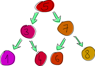
> nums = [8,6,4,1,7,3,5]
[8,6,4,1,7,3,5] : List number
> numsTree = List.foldr treeInsert EmptyTree nums
Node 5 (Node 3 (Node 1 EmptyTree EmptyTree) (Node 4 EmptyTree EmptyTree)) (Node 7 (Node 6 EmptyTree EmptyTree) (Node 8 EmptyTree EmptyTree)) : Tree number
In that foldr, treeInsert was the folding function (it takes a tree and
a list element and produces a new tree) and EmptyTree was the starting
accumulator. nums, of course, was the list we were folding over.
When we print our tree to the console, it’s not very readable, but if we try, we can make out its structure. We see that the root node is 5 and then it has two sub-trees, one of which has the root node of 3 and the other a 7, etc.
> treeElem 8 numsTree
True : Bool
> treeElem 100 numsTree
False : Bool
> treeElem 1 numsTree
True : Bool
> treeElem 10 numsTree
False : Bool
Checking for membership also works nicely. Cool.
So as you can see, algebraic data structures are a really cool and powerful concept in Elm. We can use them to make anything from boolean values and weekday enumerations to binary search trees and more!