Higher order functions

Elm functions can take functions as parameters and return functions as return values. A function that does either of those is called a higher order function. Higher order functions aren’t just a part of the Elm experience, they pretty much are the Elm experience. It turns out that if you want to define computations by defining what stuff is instead of defining steps that change some state and maybe looping them, higher order functions are indispensable. They’re a really powerful way of solving problems and thinking about programs.

Curried functions

Every function in Elm officially only takes one parameter. So how is it possible that we defined and used several functions that take more than one parameter so far? Well, it’s a clever trick! All the functions that accepted several parameters so far have been curried functions. What does that mean? You’ll understand it best on an example. Let’s take our good friend, the max function. It looks like it takes two parameters and returns the one that’s bigger. Doing max 4 5 first creates a function that takes a parameter and returns either 4 or that parameter, depending on which is bigger. Then, 5 is applied to that function and that function produces our desired result. That sounds like a mouthful but it’s actually a really cool concept. The following two calls are equivalent:

> max 4 5
5 : number
> (max 4) 5
5 : number

Putting a space between two things is simply function application. The space is sort of like an operator and it has the highest precedence. Let’s examine the type of max. It’s max : comparable -> comparable -> comparable. That can also be written as max : comparable -> (comparable -> comparable). That could be read as: max takes a comparable and returns (that’s the ->) a function that takes an comparable and returns a comparable. That’s why the return type and the parameters of functions are all simply separated with arrows.

So how is that beneficial to us? Simply speaking, if we call a function with too few parameters, we get back a partially applied function, meaning a function that takes as many parameters as we left out. Using partial application (calling functions with too few parameters, if you will) is a neat way to create functions on the fly so we can pass them to another function or to seed them with some data.

Take a look at this offensively simple function:

multThree : number -> number -> number -> number
multThree x y z = x * y * z

What really happens when we do multThree 3 5 9 or ((multThree 3) 5) 9? First, 3 is applied to multThree, because they’re separated by a space. That creates a function that takes one parameter and returns a function. So then 5 is applied to that, which creates a function that will take a parameter and multiply it by 15. 9 is applied to that function and the result is 135 or something. Remember that this function’s type could also be written as multThree : number -> (number -> (number -> number)). The thing before the -> is the parameter that a function takes and the thing after it is what it returns. So our function takes a number and returns a function of type number -> (number -> number). Similarly, this function takes a number and returns a function of type number -> number. And this function, finally, just takes a number and returns a number. Take a look at this:

> multTwoWithNine = multThree 9
<function> : number -> number -> number
> multTwoWithNine 2 3
54 : number
> multWithEighteen = multTwoWithNine 2
<function> : number -> number
> multWithEighteen 10
180 : number

By calling functions with too few parameters, so to speak, we’re creating new functions on the fly. What if we wanted to create a function that takes a number and compares it to 100? We could do something like this:

compareWithHundred : number -> Order
compareWithHundred x = compare 100 x

If we call it with 99, it returns a GT. Simple stuff. Notice that the x is on the right hand side on both sides of the equation. Now let’s think about what compare 100 returns. It returns a function that takes a number and compares it with 100. Wow! Isn’t that the function we wanted? We can rewrite this as:

compareWithHundred : number -> Order
compareWithHundred = compare 100

The type declaration stays the same, because compare 100 returns a function. Compare has a type of number -> (number -> Order) and calling it with 100 returns a number -> Order.

Yo! Make sure you really understand how curried functions and partial application work because they’re really important!

Infix functions can also be partially applied by wrapping the function in parentheses. This creates a function that takes one parameter and then applies it to the right side of the function. An insultingly trivial function:

subTen : number -> number
subTen = (-) 10

Calling, say, subTen 5 is equivalent to doing 10 - 5, as is doing ((-) 10) 5.

Some higher-orderism is in order

Functions can take functions as parameters and also return functions. To illustrate this, we’re going to make a function that takes a function and then applies it twice to something!

applyTwice : (a -> a) -> a -> a
applyTwice f x = f (f x)

First of all, notice the type declaration. Before, we didn’t need parentheses because -> is naturally right-associative. However, here, they’re mandatory. They indicate that the first parameter is a function that takes something and returns that same thing. The second parameter is something of that type also and the return value is also of the same type. We could read this type declaration in the curried way, but to save ourselves a headache, we’ll just say that this function takes two parameters and returns one thing. The first parameter is a function (of type a -> a) and the second is that same a. The function can also be Int -> Int or String -> String or whatever. But then, the second parameter also has to be of that type.

Note: From now on, we’ll say that functions take several parameters despite each function actually taking only one parameter and returning partially applied functions until we reach a function that returns a solid value. So for simplicity’s sake, we’ll say that a -> a -> a takes two parameters, even though we know what’s really going on under the hood.

The body of the function is pretty simple. We just use the parameter f as a function, applying x to it by separating them with a space and then applying the result to f again. Anyway, playing around with the function:

> applyTwice ((+) 3) 10
16 : number
> applyTwice ((++) "HAHA ") "HEY"
"HAHA HAHA HEY" : String
> applyTwice (multThree 2 2) 9
144 : number
> applyTwice ((::) 3) [1]
[3,3,1] : List number

The awesomeness and usefulness of partial application is evident. If our function requires us to pass it a function that takes only one parameter, we can just partially apply a function to the point where it takes only one parameter and then pass it.

Now we’re going to use higher order programming to implement a really useful function called zipWith. It takes a function and two lists as parameters and then joins the two lists by applying the function between corresponding elements. Here’s how we’ll implement it:

zipWith : (a -> b -> c) -> List a -> List b -> List c
zipWith f list1 list2 = case (list1, list2) of
    (_, []) -> []
    ([], _) -> []
    (x::xs, y::ys) -> f x y :: zipWith f xs ys

Look at the type declaration. The first parameter is a function that takes two things and produces a third thing. They don’t have to be of the same type, but they can. The second and third parameter are lists. The result is also a list. The first has to be a list of a’s, because the joining function takes a’s as its first argument. The second has to be a list of b’s, because the second parameter of the joining function is of type b. The result is a list of c’s. If the type declaration of a function says it accepts an a -> b -> c function as a parameter, it will also accept an a -> a -> a function, but not the other way around! Remember that when you’re making functions, especially higher order ones, and you’re unsure of the type, you can just try omitting the type declaration and then checking what Elm infers it to be using the repl.

The action in the function is pretty similar to the normal zip. The edge conditions are the same, only there’s an extra argument, the joining function, but that argument doesn’t matter in the edge conditions, so we just use a _ for it. And function body at the last pattern is also similar to zip, only it doesn’t do (x,y), but f x y. A single higher order function can be used for a multitude of different tasks if it’s general enough. Here’s a little demonstration of all the different things our zipWith function can do:

> zipWith (+) [4,2,5,6] [2,6,2,3]
[6,8,7,9] : List number
> zipWith max [6,3,2,1] [7,3,1,5]
[7,3,2,5] : List number
> zipWith (++) ["foo ", "bar ", "baz "] ["fighters", "hoppers", "aldrin"]
["foo fighters","bar hoppers","baz aldrin"] : List String
> zipWith (*) (List.repeat 5 2) [1, 2, 3, 4, 5, 6, 7, 8, 9, 10]
[2,4,6,8,10] : List number
> zipWith (zipWith (*)) [[1,2,3],[3,5,6],[2,3,4]] [[3,2,2],[3,4,5],[5,4,3]]
[[3,4,6],[9,20,30],[10,12,12]] : List (List number)

As you can see, a single higher order function can be used in very versatile ways. Imperative programming usually uses stuff like for loops, while loops, setting something to a variable, checking its state, etc. to achieve some behavior and then wrap it around an interface, like a function. Functional programming uses higher order functions to abstract away common patterns, like examining two lists in pairs and doing something with those pairs or getting a set of solutions and eliminating the ones you don’t need.

We’ll implement another function that’s already in the standard library, called flip. flip simply takes a function and returns a function that is like our original function, only the first two arguments are flipped. We can implement it like so:

flip : (a -> b -> c) -> (b -> a -> c)
flip f y x =
    let
        g = f
    in
        g x y

Reading the type declaration, we say that it takes a function that takes an a and a b and returns a function that takes a b and an a. But because functions are curried by default, the second pair of parentheses is really unnecessary, because -> is right associative by default. (a -> b -> c) -> (b -> a -> c) is the same as (a -> b -> c) -> (b -> (a -> c)), which is the same as (a -> b -> c) -> b -> a -> c. We wrote that g x y = f y x. If that’s true, then f y x = g x y must also hold, right? Keeping that in mind, we can define this function in an even simpler manner.

flip : (a -> b -> c) -> b -> a -> c
flip f y x = f x y

Here, we take advantage of the fact that functions are curried. When we call flip f without the parameters y and x, it will return an f that takes those two parameters but calls them flipped. Even though flipped functions are usually passed to other functions, we can take advantage of currying when making higher-order functions by thinking ahead and writing what their end result would be if they were called fully applied.

> flip (List.map2 (,)) [ 1, 2, 3, 4, 5 ] (String.toList "hello")
[('h',1),('e',2),('l',3),('l',4),('o',5)] : List ( Char, number )
> zipWith (flip (/)) (List.repeat 5 2) [10,8,6,4,2]
[5,4,3,2,1] : List : Float

Maps and filters

map takes a function and a list and applies that function to every element in the list, producing a new list. Let’s see what its type signature is and how it’s defined.

map : (a -> b) -> List a -> List b
map f list = case list of
    [] -> []
    (x::xs) -> f x :: map f xs

The type signature says that it takes a function that takes an a and returns a b, a list of a’s and returns a list of b’s. It’s interesting that just by looking at a function’s type signature, you can sometimes tell what it does. map is one of those really versatile higher-order functions that can be used in millions of different ways. Here it is in action:

> List.map ((+) 3) [1,5,3,1,6]
[4,8,6,4,9] : List number
> List.map (flip (++) "!") ["BIFF", "BANG", "POW"]
["BIFF!","BANG!","POW!"] : List String
> List.map (List.repeat 3) [3, 4, 5, 6]
[[3,3,3],[4,4,4],[5,5,5],[6,6,6]] : List (List number)
> List.map (List.map (flip (^) 2)) [[1,2],[3,4,5,6],[7,8]]
[[1,4],[9,16,25,36],[49,64]] : List (List number)
> List.map Tuple.first [(1,2),(3,5),(6,3),(2,6),(2,5)]
[1,3,6,2,2] : List number

filter is a function that takes a predicate (a predicate is a function that tells whether something is true or not, so in our case, a function that returns a boolean value) and a list and then returns the list of elements that satisfy the predicate. The type signature and implementation go like this:

filter : (a -> Bool) -> List a -> List a
filter p list = case list of
    [] -> []

    (x::xs) ->
        if p x then
            x :: filter p xs
        else
            filter p xs

Pretty simple stuff. If p x evaluates to True, the element gets included in the new list. If it doesn’t, it stays out. Some usage examples:

> List.filter ((<) 3) [1,5,3,2,1,6,4,3,2,1]
[5,6,4] : List number
> List.filter ((==) 3) [1,2,3,4,5]
[3] : List number
> List.filter (let nonEmpty ls = not (List.isEmpty ls) in nonEmpty) \
|    [[1,2,3],[],[3,4,5],[2,2],[],[],[]]
[[1,2,3],[3,4,5],[2,2]] : List (List number)

Mapping and filtering is the bread and butter of every functional programmer’s toolbox. Recall how we solved the problem of finding right triangles with a certain circumference. With imperative programming, we would have solved it by nesting three loops and then testing if the current combination satisfies a right triangle and if it has the right perimeter. If that’s the case, we would have printed it out to the screen or something. In functional programming, that pattern is achieved with mapping and filtering. You make a function that takes a value and produces some result. We map that function over a list of values and then we filter the resulting list out for the results that satisfy our search.

Let’s find the largest number under 100,000 that’s divisible by 3829. To do that, we’ll just filter a set of possibilities in which we know the solution lies.

largestDivisible : Maybe Int
largestDivisible =
    let
        p x = x % 3829 == 0
    in
    List.head (List.filter p List.reverse (List.range 0 99999))

We first make a list of all numbers between 0 and 100,000, descending. Then we filter it by our predicate and because the numbers are sorted in a descending manner, the largest number that satisfies our predicate is the first element of the filtered list.

Next up, we’re going to find the sum of all odd squares that are smaller than 10,000. But first, because we’ll be using it in our solution, we’re going to introduce the takeWhile function. It takes a predicate and a list and then goes from the beginning of the list and returns its elements while the predicate holds true. Once an element is found for which the predicate doesn’t hold, it stops. If we wanted to get all square numbers less than 100, we could do (takeWhile (flip (<) 100) (List.map (flip (^) 2) (List.range 0 100)) and it would return a list of all square numbers less than 100.

takeWhile is defined like this:

takeWhile : (a -> Bool) -> List a -> List a
takeWhile p list = case list of
    [] -> []
    (x::xs) -> if p x then x :: takeWhile p xs else []

Okay. The sum of all odd squares that are smaller than 10,000. First, we’ll begin by mapping the (flip (^) 2) function to the list List.range 0 9999. Then we filter them so we only get the odd ones. Finally, we’ll get the sum of that list. We don’t even have to define a function for that, we can do it in one line in Elm:

> List.sum (takeWhile (flip (<) 10000) (List.filter (\n -> n % 2 /= 0) \
|    (List.map (flip (^) 2) (List.range 0 10000))))
166650 : Int

Awesome! We start with some initial data and then we map over it, filter it and cut it until it suits our needs and then we just sum it up.

For our next problem, we’ll be dealing with Collatz sequences. We take a natural number. If that number is even, we divide it by two. If it’s odd, we multiply it by 3 and then add 1 to that. We take the resulting number and apply the same thing to it, which produces a new number and so on. In essence, we get a chain of numbers. It is thought that for all starting numbers, the chains finish at the number 1. So if we take the starting number 13, we get this sequence: 13, 40, 20, 10, 5, 16, 8, 4, 2, 1. 13*3 + 1 equals 40. 40 divided by 2 is 20, etc. We see that the chain has 10 terms.

Now what we want to know is this: for all starting numbers between 1 and 100, how many chains have a length greater than 15? First off, we’ll write a function that produces a chain:

chain : Int -> List Int
chain n = 
    let
        even n = n % 2 == 0
    in
    case n of
        1 -> [1]
        n ->
            if even n then 
                n :: chain (n // 2)
            else 
                n :: chain (n * 3 + 1)

Because the chains end at 1, that’s the edge case. This is a pretty standard recursive function.

> chain 10
[10,5,16,8,4,2,1] : List number
> chain 1
[1] : List number
> chain 30
[30,15,46,23,70,35,106,53,160,80,40,20,10,5,16,8,4,2,1] : List number

Yay! It seems to be working correctly. And now, the function that tells us the answer to our question:

numLongChains : Int
numLongChains = 
    let
        isLong xs = List.length xs > 15
    in
    List.length (List.filter isLong (List.map chain (List.range 1 100)))

We map the chain function to List.range 1 100 to get a list of chains, which are themselves represented as lists. Then, we filter them by a predicate that just checks whether a list’s length is longer than 15. Once we’ve done the filtering, we see how many chains are left in the resulting list.

Using map, we can also do stuff like List.map (*) (List.range 0 100), if not for any other reason than to illustrate how currying works and how (partially applied) functions are real values that you can pass around to other functions or put into lists. So far, we’ve only mapped functions that take one parameter over lists, like List.map ((*) 2) (List.range 0 5) to get a list of type List number, but we can also do List.map (*) (List.range 0 5) without a problem. What happens here is that the number in the list is applied to the function *, which has a type of number -> number -> number. Applying only one parameter to a function that takes two parameters returns a function that takes one parameter. If we map * over the list List.range 0 5, we get back a list of functions that only take one parameter, so List (number -> number). List.map (*) (List.range 0 5) produces a list like the one we’d get by writing [((*) 0),((*) 1),((*) 2),((*) 3),((*) 4),((*) 5)]

> let \
|     listOfFuns = List.map (*) (List.range 0 5) \
| in \
|     List.map (\f -> f 2) listOfFuns 
[0,2,4,6,8,10] : List Int

Mapping over the list of functions, applying each partial function with the value 2, produces a list of values where each item in the list is the product of the initial value (from the range 0 to 5) multiplied by 2. We used a lambda function to help us apply our partial functions, which we’ll talk more about in the next section. We could also have used the function application operator (|>) to achieve the same effect.

Definitely Maybe

Let’s take a quick detour to talk about the Maybe type. We’ve already seen a few examples that returned this type (and we’re about to see a whole lot more), but we haven’t yet explained what it is. First, let’s look at how the Maybe type is defined:

type Maybe a
    = Just a
    | Nothing

So Maybe is a polymorphic type which is either Just a, or Nothing. How is this useful? Many programming problems have edge cases where there is no well-defined answer. In such cases, we can say that we’re dealing with a partial function (as opposed to a total function), because the domain of our function (the inputs) only partially maps to the codomain (an output). In other words, there are values in our domain for which the function does not produce a value in the codomain. In other, other words, there are inputs to our function which are technically valid (from a type perspective), but which can’t produce an output that really makes any sense. Let’s take the example of List.head. Unsurprisingly, this function takes a list, and returns its head. But what should we return in the case of the empty list? An empty list can’t really be said to have a head… or a tail for that matter. In some languages, this might be handled by throwing a runtime exception (Elm strives to eliminate all runtime exceptions). In others, this might be handled by returning a Null value. With null values, the programmer must take extra care to check whether their return value is null before they try to use it. If they don’t, again we’re likely to see runtime exceptions. The way Elm handles this, while avoiding those pesky runtime exceptions, is to encode this uncertainty into a type. With the Maybe type, the (non-)existence of a value is reflected plainly and completely in the type, and we’re forced to handle the case where we don’t get back any meaningful value. To demonstrate this, let’s look at how head is implemented.

head : List a -> Maybe a
head list = case list of
    [] -> Nothing
    (x::xs) -> Just x

If we have an empty list, we return Nothing, otherwise we get Just x, where x is the head of the list. Whenever we have a Maybe type, we can pattern match against both cases. For example:

> case List.head [1,2,3] of \
|    Nothing -> "Empty!" \
|    Just a -> "Yay! The head value is: " ++ toString a
"Yay! The head value is: 1" : String

And because the Elm compiler will complain if we don’t handle every possibility, we can always be certain that we have handled all of the edge cases.

So, does that make sense? If you answered ‘maybe’, then you’re ready to continue.

Lambdas

Lambdas are basically anonymous functions that are used because we need some functions only once. Normally, we make a lambda with the sole purpose of passing it to a higher-order function. To make a lambda, we write a \ (because it kind of looks like the greek letter lambda if you squint hard enough) and then we write the parameters, separated by spaces. After that comes a -> and then the function body. We usually surround them by parentheses, because otherwise they extend all the way to the right.

If you look back a few paragraphs, you’ll see that we used a let binding in our numLongChains function to make the isLong function for the sole purpose of passing it to List.filter. Well, instead of doing that, we can use a lambda:

numLongChains : Int
numLongChains = List.length (List.filter (\xs -> List.length xs > 15)
    (List.map chain (List.range 1 100)))

Lambdas are expressions, that’s why we can just pass them like that. The expression (\xs -> List.length xs > 15) returns a function that tells us whether the length of the list passed to it is greater than 15.

People who are not well acquainted with how currying and partial application works often use lambdas where they don’t need to. For instance, the expressions List.map ((+) 3) [1,6,3,2] and List.map (\x -> x + 3) [1,6,3,2] are equivalent since both ((+) 3) and (\x -> x + 3) are functions that take a number and add 3 to it. Needless to say, making a lambda in this case is stupid since using partial application is much more readable.

Like normal functions, lambdas can take any number of parameters:

zipWith (\a b -> (a * 30 + 3) / b) [5,4,3,2,1] [1,2,3,4,5]
[153.0,61.5,31.0,15.75,6.6]

And like normal functions, you can pattern match in lambdas. The only difference is that you can’t define several patterns for one parameter, like making a [] and a (x:xs) pattern for the same parameter and then having values fall through. If the pattern does not cover all possible inputs, it will fail to compile.

List.map (\(a,b) -> a + b) [(1,2),(3,5),(6,3),(2,6),(2,5)]
[3,8,9,8,7]

Lambdas are normally surrounded by parentheses unless we mean for them to extend all the way to the right. Here’s something interesting: due to the way functions are curried by default, these two are equivalent:

addThree : number -> number -> number -> number
addThree x y z = x + y + z

addThree : number -> number -> number -> number
addThree = \x -> \y -> \z -> x + y + z

If we define a function like this, it’s obvious why the type declaration is what it is. There are three ->’s in both the type declaration and the equation. But of course, the first way to write functions is far more readable, the second one is pretty much a gimmick to illustrate currying.

However, there are times when using this notation is cool. I think that the flip function is the most readable when defined like so:

flip : (a -> b -> c) -> b -> a -> c
flip f = \x y -> f y x

Even though that’s the same as writing flip f x y = f y x, we make it obvious that this will be used for producing a new function most of the time. The most common use case with flip is calling it with just the function parameter and then passing the resulting function on to a map or a filter. So use lambdas in this way when you want to make it explicit that your function is mainly meant to be partially applied and passed on to a function as a parameter.

Only folds and horses

Back when we were dealing with recursion, we noticed a theme throughout many of the recursive functions that operated on lists. Usually, we’d have an edge case for the empty list. We’d introduce the x::xs pattern and then we’d do some action that involves a single element and the rest of the list. It turns out this is a very common pattern, so a couple of very useful functions were introduced to encapsulate it. These functions are called folds. They’re sort of like the map function, only they reduce the list to some single value.

A fold takes a binary function, a starting value (I like to call it the accumulator) and a list to fold up. The binary function itself takes two parameters. The binary function is called with the accumulator and the first (or last) element and produces a new accumulator. Then, the binary function is called again with the new accumulator and the now new first (or last) element, and so on. Once we’ve walked over the whole list, only the accumulator remains, which is what we’ve reduced the list to.

First let’s take a look at the foldl function, also called the left fold. It folds the list up from the left side. The binary function is applied between the starting value and the head of the list. That produces a new accumulator value and the binary function is called with that value and the next element, etc.

Let’s implement sum again, only this time, we’ll use a fold instead of explicit recursion.

sum : List number -> number
sum xs = List.foldl (\x acc -> acc + x) 0 xs

Testing, one two three:

sum [3,5,2,1]
11

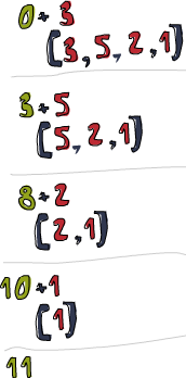
Let’s take an in-depth look into how this fold happens. \x acc -> acc + x is the binary function. 0 is the starting value and xs is the list to be folded up. Now first, 0 is used as the acc parameter to the binary function and 3 is used as the x (or the current element) parameter. 0 + 3 produces a 3 and it becomes the new accumulator value, so to speak. Next up, 3 is used as the accumulator value and 5 as the current element and 8 becomes the new accumulator value. Moving forward, 8 is the accumulator value, 2 is the current element, the new accumulator value is 10. Finally, that 10 is used as the accumulator value and 1 as the current element, producing an 11. Congratulations, you’ve done a fold!

This professional diagram on the left illustrates how a fold happens, step by step (day by day!). The greenish brown number is the accumulator value. You can see how the list is sort of consumed up from the left side by the accumulator. Om nom nom nom! If we take into account that functions are curried, we can write this implementation ever more succinctly, like so:

sum : List number -> number
sum = List.foldl (+) 0

The lambda function (\x acc -> acc + x) is the same as (+). We can omit the xs as the parameter because calling List.foldl (+) 0 will return a function that takes a list. Generally, if you have a function like foo a = bar b a, you can rewrite it as foo = bar b, because of currying.

Anyhoo, let’s implement another function with a left fold before moving on to right folds. I’m sure you all know that List.member checks whether a value is part of a list so I won’t go into that again (whoops, just did!). Let’s implement it with a left fold.

member : a -> List a -> Bool
member y ys = List.foldl (\x acc -> if x == y then True else acc) False ys

Well, well, well, what do we have here? The starting value and accumulator here is a boolean value. The type of the accumulator value and the end result is always the same when dealing with folds. Remember that if you ever don’t know what to use as a starting value, it’ll give you some idea. We start off with False. It makes sense to use False as a starting value. We assume it isn’t there. Also, if we call a fold on an empty list, the result will just be the starting value. Then we check the current element is the element we’re looking for. If it is, we set the accumulator to True. If it’s not, we just leave the accumulator unchanged. If it was False before, it stays that way because this current element is not it. If it was True, we leave it at that.

The right fold, foldr works in a similar way to the left fold, only the accumulator eats up the values from the right.

The accumulator value (and hence, the result) of a fold can be of any type. It can be a number, a boolean or even a new list. We’ll be implementing the map function with a right fold. The accumulator will be a list, we’ll be accumulating the mapped list element by element. From that, it’s obvious that the starting element will be an empty list.

map : (a -> b) -> List a -> List b
map f xs = List.foldr (\x acc -> f x :: acc) [] xs

If we’re mapping ((+) 3) to [1,2,3], we approach the list from the right side. We take the last element, which is 3 and apply the function to it, which ends up being 6. Then, we prepend it to the accumulator, which is []. 6::[] is [6] and that’s now the accumulator. We apply ((+) 3) to 2, that’s 5 and we prepend (::) it to the accumulator, so the accumulator is now [5,6]. We apply ((+) 3) to 1 and prepend that to the accumulator and so the end value is [4,5,6].

Of course, we could have implemented this function with a left fold too. It would be map f xs = List.foldl (\x acc -> acc ++ [f x]) [] xs, but the thing is that the ++ function is much more expensive than ::, so we usually use right folds when we’re building up new lists from a list.

If you reverse a list, you can do a right fold on it just like you would have done a left fold and vice versa. Sometimes you don’t even have to do that. The sum function can be implemented pretty much the same with a left and right fold.

Folds can be used to implement any function where you traverse a list once, element by element, and then return something based on that. Whenever you want to traverse a list to return something, chances are you want a fold. That’s why folds are, along with maps and filters, one of the most useful types of functions in functional programming.

Just to show you how powerful folds are, we’re going to implement a bunch of standard library functions by using folds:

maximum : List a -> Maybe a
maximum = List.foldr
    (\x acc ->
        if
            case acc of
                Nothing -> True
                Just n -> x > n
        then
            Just x
        else
            acc)
    Nothing

reverse : List a -> List a
reverse = List.foldl (\x acc -> x :: acc) []

product : List a -> a
product = List.foldr (*) 1

filter : (a -> Bool) -> List a -> List a
filter p = List.foldr (\x acc -> if p x then x :: acc else acc) []

head : List a -> Maybe a
head = List.foldr (\x _ -> Just x) Nothing

last : List a -> Maybe a
last = List.foldl (\x _ -> Just x) Nothing

head is better implemented by pattern matching, but this just goes to show, you can still achieve it by using folds. Our reverse definition is pretty clever, I think. We take a starting value of an empty list and then approach our list from the left and just prepend to our accumulator. In the end, we build up a reversed list. \x acc -> x :: acc kind of looks like the :: function, only the parameters are flipped. That’s why we could have also written our reverse as foldl (flip (::)) [].

Another way to picture right and left folds is like this: say we have a right fold and the binary function is f and the starting value is z. If we’re right folding over the list [3,4,5,6], we’re essentially doing this: f 3 (f 4 (f 5 (f 6 z))). f is called with the last element in the list and the accumulator, that value is given as the accumulator to the next to last value and so on. If we take f to be + and the starting accumulator value to be 0, that’s 3 + (4 + (5 + (6 + 0))). Or if we write + as a prefix function, that’s (+) 3 ((+) 4 ((+) 5 ((+) 6 0))). Similarly, doing a left fold over that list with g as the binary function and z as the accumulator is the equivalent of g (g (g (g z 3) 4) 5) 6. If we use flip (::) as the binary function and [] as the accumulator (so we’re reversing the list), then that’s the equivalent of flip (::) (flip (::) (flip (::) (flip (::) [] 3) 4) 5) 6. And sure enough, if you evaluate that expression, you get [6,5,4,3].

scanl is like foldl, only it reports all the intermediate accumulator states in the form of a list.

> List.scanl (+) 0 [3,5,2,1]
[0,3,8,10,11] : List number
List.scanl (::) [] [3,2,1]
[[],[3],[2,3],[1,2,3]] : List (List number)

When using a scanl, the final result will be in the last element of the resulting list.

Scans are used to monitor the progression of a function that can be implemented as a fold. Let’s answer us this question: How many elements does it take for the sum of the roots of all natural numbers to exceed 1000? To get the squares of all natural numbers, we just do List.map sqrt (List.map toFloat (List.range 1 1000)) Now, to get the sum, we could do a fold, but because we’re interested in how the sum progresses, we’re going to do a scan. Once we’ve done the scan, we just see how many sums are under 1000. The first sum in the scanlist will be 1, normally. The second will be 1 plus the square root of 2. The third will be that plus the square root of 3. If there are X sums under 1000, then it takes X+1 elements for the sum to exceed 1000.

sqrtSums : Int
sqrtSums =
    let
        sqrts = List.map sqrt (List.map toFloat (List.range 1 1000))
    in
    List.length (takeWhile (flip (<) 1000) (List.scanl (+) 1 sqrts))

> sqrtSums
131 : Int
> List.sum (List.map sqrt (List.map toFloat (List.range 1 131)))
1005.0942035344083 : Float
> List.sum (List.map sqrt (List.map toFloat (List.range 1 130)))
993.6486803921487 : Float

Function application with |> and <|

Alright, next up, we’ll take a look at the |> and <| functions, also called forward and backward function application, respectively. First of all, let’s check out how they’re defined:

(|>) : a -> (a -> b) -> b
(|>) x f =
    f x

(<|) : (a -> b) -> a -> b
(<|) f x =
    f x

What the heck? What are these useless operators? It’s just function application! Well, almost, but not quite! Whereas normal function application (putting a space between two things) has a really high precedence, the |> and <| functions have the lowest precedence. Function application with a space is left-associative (so f a b c is the same as ((f a) b) c)), function application with |> and <| are right-associative.

That’s all very well, but how does this help us? Most of the time, it’s a convenience function so that we don’t have to write so many parentheses. Consider the expression List.sum (List.map sqrt (List.map toFloat (List.range 1 130))). Because <| has such a low precedence, we can rewrite that expression as List.sum <| List.map sqrt <| List.map toFloat <| List.range 1 130, saving ourselves precious keystrokes! When a <| is encountered, the expression on its right is applied as the parameter to the function on its left. How about sqrt 3 + 4 + 9? This adds together 9, 4 and the square root of 3. If we want get the square root of 3 + 4 + 9, we’d have to write sqrt (3 + 4 + 9) or if we use <| we can write it as sqrt <| 3 + 4 + 9 because <| has the lowest precedence of any operator. That’s why you can imagine a <| being sort of the equivalent of writing an opening parentheses and then writing a closing one on the far right side of the expression.

How about List.sum (List.filter ((>) 10) (List.map ((*) 2) (List.range 2 10)))? Well, because <| is right-associative, f (g (z x)) is equal to f <| g <| z x. And so, we can rewrite List.sum (List.filter ((>) 10) (List.map ((*) 2) (List.range 2 10))) as List.sum <| List.filter ((>) 10) <| List.map ((*) 2) <| List.range 2 10.

Forward function application behaves similarly, but values are applied from the other direction.

> List.sum [3, 7, 6] |> sqrt |> List.repeat 3 |> List.map ((+) 2)
[6,6,6] : List Float

In the example above, the result of List.sum [3, 7, 6] (16) is passed to the sqrt function, which produces 4.0, which is passed to List.repeat 3, which produces the list [4,4,4], which is passed to List.map ((+) 2), which produces the final result [6,6,6]`.

But apart from getting rid of parentheses, <| and |> mean that function application can be treated just like another function. That way, we can, for instance, map function application over a list of functions.

> List.map ((|>) 3) [((+) 4), ((*) 10), (flip (^) 2), sqrt]
[7,30,9,1.7320508075688772] : List Float

Function composition

In mathematics, function composition is defined like this: , meaning that composing two functions produces a new function that, when called with a parameter, say, x is the equivalent of calling g with the parameter x and then calling the f with that result.

In Elm, function composition is pretty much the same thing. We do function composition with the << and >> functions, which are defined like so:

(<<) : (b -> c) -> (a -> b) -> (a -> c)
(<<) g f x =
    g (f x)

(>>) : (a -> b) -> (b -> c) -> (a -> c)
(>>) f g x =
    g (f x)

Mind the type declarations. Focusing on the first example (<<) g must take as its parameter a value that has the same type as f’s return value. So the resulting function takes a parameter of the same type that f takes and returns a value of the same type that g returns. The expression negate << ((*) 3) returns a function that takes a number, multiplies it by 3 and then negates it.

One of the uses for function composition is making functions on the fly to pass to other functions. Sure, we can use lambdas for that, but many times, function composition is clearer and more concise. Say we have a list of numbers and we want to turn them all into negative numbers. One way to do that would be to get each number’s absolute value and then negate it, like so:

> List.map (\x -> negate (abs x)) [5,-3,-6,7,-3,2,-19,24]
[-5,-3,-6,-7,-3,-2,-19,-24] : List number

Notice the lambda and how it looks like the result function composition. Using function composition, we can rewrite that as:

> List.map (negate << abs) [5,-3,-6,7,-3,2,-19,24]
[-5,-3,-6,-7,-3,-2,-19,-24] : List number

Fabulous! Function composition is right-associative, so we can compose many functions at a time. The expression f (g (z x)) is equivalent to (f << g << z) x. With that in mind, we can turn

> List.map (\xs -> negate (List.sum (List.take 2 xs))) \
|    [List.range 1 5,List.range 3 6,List.range 1 7]
[-3,-7,-3] : List Int

into

> List.map (negate << List.sum << List.take 2) \
|    [List.range 1 5,List.range 3 6,List.range 1 7] 
[-3,-7,-3] : List Int

But what about functions that take several parameters? Well, if we want to use them in function composition, we usually have to partially apply them just so much that each function takes just one parameter. List.sum (List.repeat 5 (max 6.7 8.9)) can be rewritten as (List.sum << List.repeat 5 << max 6.7) 8.9 or as List.sum << List.repeat 5 << max 6.7 <| 8.9. What goes on in here is this: a function that takes what max 6.7 takes and applies List.repeat 5 to it is created. Then, a function that takes the result of that and does a List.sum of it is created. Finally, that function is called with 8.9. But normally, you just read that as: apply 8.9 to max 6.7, then apply List.repeat 5 to that and then apply List.sum to that. If you want to rewrite an expression with a lot of parentheses by using function composition, you can start by putting the last parameter of the innermost function after a <| and then just composing all the other function calls, writing them without their last parameter and putting << between them. If you have List.repeat 100 (List.product (List.map ((*) 3) (List.map2 max [1,2,3,4,5] [4,5,6,7,8]))), you can write it as List.repeat 100 << List.product << List.map ((*) 3) << List.map2 max [1,2,3,4,5] <| [4,5,6,7,8]. If the expression ends with three parentheses, chances are that if you translate it into function composition, it’ll have three composition operators.

Another common use of function composition is defining functions in the so-called point free style (also called the pointless style). Take for example this function that we wrote earlier:

sum : List number -> number
sum xs = List.foldl (+) 0 xs

The xs is exposed on both right sides. Because of currying, we can omit the xs on both sides, because calling List.foldl (+) 0 creates a function that takes a list. Writing the function as sum = List.foldl (+) 0 is called writing it in point free style. How would we write this in point free style?

fn x = ceiling (negate (tan (cos (max 50 x))))

We can’t just get rid of the x on both right right sides. The x in the function body has parentheses after it. cos (max 50) wouldn’t make sense. You can’t get the cosine of a function. What we can do is express fn as a composition of functions.

fn = ceiling << negate << tan << cos << max 50

Excellent! Many times, a point free style is more readable and concise, because it makes you think about functions and what kind of functions composing them results in instead of thinking about data and how it’s shuffled around. You can take simple functions and use composition as glue to form more complex functions. However, many times, writing a function in point free style can be less readable if a function is too complex. That’s why making long chains of function composition is discouraged, although I plead guilty of sometimes being too composition-happy. The prefered style is to use let bindings to give labels to intermediary results or split the problem into sub-problems and then put it together so that the function makes sense to someone reading it instead of just making a huge composition chain.

In the section about maps and filters, we solved a problem of finding the sum of all odd squares that are smaller than 10,000. Here’s what the solution looks like when put into a function.

oddSquareSum : Int
oddSquareSum = 
    let
        odd n = n % 2 == 1
    in
    List.sum (takeWhile (flip (<) 10000)
        (List.filter odd (List.map (flip (^) 2) (List.range 1 9999))))

Being such a fan of function composition, I would have probably written that like this:

oddSquareSum : Int
oddSquareSum = 
    let
        odd n = n % 2 == 1
    in
    List.sum << takeWhile (flip (<) 10000)
        << List.filter odd << List.map (flip (^) 2) <| List.range 1 9999

However, if there was a chance of someone else reading that code, I would have written it like this:

oddSquareSum : Int
oddSquareSum =
    let
        odd n = n % 2 == 1
        oddSquares = List.filter odd <| List.map (flip (^) 2) (List.range 1 9999)
        belowLimit = takeWhile (flip (<) 10000) oddSquares
    in
        List.sum belowLimit

It wouldn’t win any code golf competition, but someone reading the function will probably find it easier to read than a composition chain.